Likelihood & MLE

Probability and likelihood are the same formula read in opposite directions, and that distinction is the hinge of all statistical machine learning. This page builds maximum likelihood estimation, shows why maximizing likelihood becomes minimizing your loss function, and works the three canonical MLE derivations.

Rapid Recall

Probability fixes the parameter and varies the data (summing to one); likelihood fixes the data and varies the parameter (it does not sum to one), and estimation lives on the likelihood side. Maximum likelihood picks the parameter making the observed data most probable, \(\hat\theta=\arg\max L(\theta)\). The log trick turns the product into a sum, fixing underflow and differentiation while leaving the peak unmoved. Because optimizers minimize, the negative log-likelihood is the loss: Gaussian targets give mean squared error, categorical targets give cross-entropy. The worked MLEs give the sample proportion, the sample mean, and a variance that divides by \(n\) (hence biased).

§3 Probability vs Likelihood

Probability and likelihood use the identical function, read in two opposite directions. The confusion is almost always caused by using one formula for both without being told you are reading it backwards. Every probability model has two inputs: \(\theta\) the parameters that define which distribution you have (describes the world), and \(x\) the data, the actual outcomes (what the world produced). One function ties them:

\[f(x \,;\, \theta) \quad\text{the function } f \text{, of data } x \text{, given parameter } \theta\]

Probability: fix \(\theta\), let \(x\) vary. The forward direction: the parameter is known, and you ask how likely various data outcomes are. Hold \(\theta\) fixed ("this coin is fair, \(\theta=0.5\)"), let \(x\) vary. The world is settled; the data is the unknown. As a function of \(x\), it is a proper distribution and integrates or sums to 1.

Likelihood: fix \(x\), let \(\theta\) vary. The backward direction: the data is known, and you ask how well various parameter values explain it. You have already seen the data (7 heads in 10 flips, locked); now \(\theta\) varies. You are standing after the data exists, reasoning back about what world produced it. This is the mode of estimation.

\[L(\theta \,;\, x) = f(x\,;\,\theta) \quad\text{same } f \text{, now read as a function of } \theta\]

A probability (as a function of \(x\)) sums or integrates to 1. A likelihood (as a function of \(\theta\)) does not have to, and generally does not. So likelihood is not "the probability of \(\theta\)," it is an unnormalized plausibility score used to compare \(\theta\) values against each other.

Same formula, opposite readings, the coin. Binomial: getting \(k\) heads in \(n\) flips with bias \(\theta\):

\[f(k\,;\,\theta)=\binom{n}{k}\theta^k(1-\theta)^{n-k}\]

Reading	Fix	Vary	Question	Sums to 1?
Probability	\(\theta=0.5\)	\(k=0,1,\dots,10\)	how likely is each number of heads under a fair coin?	Yes (over \(k\))
Likelihood	\(k=7\)	\(\theta\in[0,1]\)	how well does each bias explain my 7 heads?	No (over \(\theta\))

Numerical comparison. Probability (\(\theta=0.5\) fixed): \(P(7)=120\cdot 0.5^{10}\approx 0.117\), \(P(5)=252\cdot0.5^{10}\approx0.246\). Summed over all \(k\): exactly 1. Likelihood (data = 7 heads fixed):

• \(L(\theta=0.5)=120\cdot0.5^{7}\cdot0.5^{3}\approx 0.117\)
• \(L(\theta=0.7)=120\cdot0.7^{7}\cdot0.3^{3}\approx 0.267\) (highest)
• \(L(\theta=0.9)=120\cdot0.9^{7}\cdot0.1^{3}\approx 0.057\)

Two things: \(L(\theta{=}0.5)=0.117\) is the exact same number as \(P(7\,|\,\theta{=}0.5)\), same formula, different question. And the peak sits at \(\theta=0.7\), matching the intuition that 7/10 heads is best explained by a coin of bias 0.7.

The likelihood of theta given 7 heads in 10 flips, peaking at the maximum likelihood estimate 0.7.

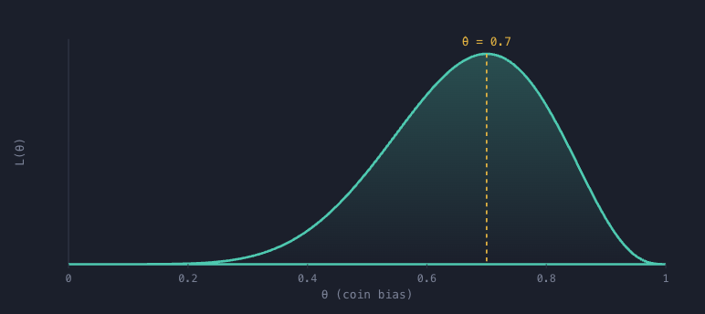
The bridge to estimation. Maximum Likelihood Estimation (MLE) is the formal version of "find the \(\theta\) that best explains the data": slide \(\theta\) across all values, compute the likelihood, pick the peak.

\[\hat{\theta}_{\text{MLE}} = \arg\max_{\theta} \; L(\theta\,;\,x)\]

Probability: "I know the dice. What rolls should I expect?" World fixed, data varies, sums to 1. Likelihood: "I saw the rolls. What dice were probably in play?" Data fixed, world varies, does not sum to 1. Probability slices the joint function along the data axis; likelihood slices it along the parameter axis. One predicts; the other infers. Estimation lives entirely on the likelihood side.

§4 Why theta, Why Likelihood, Why Maximize It, and Why It Becomes the Loss

This is the spine of statistical machine learning, built in four linked steps.

Step 1, why do we even care about theta?

Because theta is the model. When you say "I have a model," what you concretely possess is a distribution with parameters \(\theta\). Pin down \(\theta\) and you have pinned down the entire distribution:

• Predict. Known \(\theta\) lets you compute the probability of any future outcome.
• Understand. \(\theta\) often is the question, "average drug effect" is \(\mu\); "fraction who churn" is \(p\).
• Compress. 10 million points, if they follow a known family, collapse to a handful of numbers.

In pure frequentist estimation, \(\theta\) is a fixed unknown constant and we produce a single best guess \(\hat\theta\). The idea that \(\theta\) itself has a distribution is the Bayesian view. MLE lives in the frequentist world: \(\theta\) is one true fixed value we are hunting.

Step 2, why likelihood is the right instrument

Estimation runs backward: data fixed, \(\theta\) varies, and likelihood scores how well each candidate \(\theta\) explains the observed data, \(L(\theta)=f(\text{data};\theta)\). All the information the data carries about \(\theta\) is contained in the likelihood function. The data we observed actually happened; a good explanation should assign it reasonably high probability. If some \(\theta\) makes our observed data wildly improbable, it is a poor explanation; if another makes it look natural, it is a good one. Likelihood quantifies "how unsurprised would this \(\theta\) be by what we saw."

Step 3, why maximize the likelihood?

Of all possible worlds, choose the one under which the data we actually observed is most probable. Almost tautologically the most defensible single guess: any other choice goes with a world that explains your evidence worse than an available alternative, irrational with no extra information.

\[\hat{\theta}_{\text{MLE}} = \arg\max_{\theta} L(\theta)\]

Why this is principled, not arbitrary. The MLE has provably good large-sample properties:

• Consistency: as \(n\to\infty\), \(\hat\theta_{\text{MLE}}\to\) true \(\theta\).
• Asymptotic efficiency: lowest possible variance in the large-sample limit (hits the Cramer-Rao bound).
• Asymptotic normality: \(\hat\theta_{\text{MLE}}\) becomes normal around true \(\theta\), what lets you build CIs and tests on top.
• Invariance: if \(\hat\theta\) is the MLE of \(\theta\), then \(g(\hat\theta)\) is the MLE of \(g(\theta)\) for any \(g\).

Step 4, the mechanics and the log trick

For \(n\) independent points, independence factorizes the joint probability into a product:

\[L(\theta) = f(x_1,\dots,x_n;\theta) = \prod_{i=1}^{n} f(x_i;\theta)\]

This product is a nightmare: (1) numerical underflow, each \(f<1\), multiply 10,000 of them and you get \(10^{-30000}\), rounded to 0; (2) differentiation hell, the product rule cascaded \(n\) times; (3) no clean algebra. Take the log. Define the log-likelihood:

\[\ell(\theta) = \log L(\theta) = \log\prod_{i=1}^{n} f(x_i;\theta) = \sum_{i=1}^{n}\log f(x_i;\theta)\]

The single magic step, \(\log(\text{product})=\text{sum of logs}\), fixes all three: sums of logs do not underflow, the derivative of a sum is the sum of derivatives, and logs turn exponents into multipliers (gold for the normal, exponential, Poisson, Bernoulli). \(\log\) is monotonically increasing: if \(a>b\) then \(\log a>\log b\). Order is preserved, so the \(\theta\) that maximizes \(L\) is the exact same \(\theta\) that maximizes \(\log L\). The peak does not move, you squash the y-axis, not shift the location of the maximum.

\[\arg\max_\theta L(\theta) = \arg\max_\theta \log L(\theta)\]

Step 5, why MLE is your ML loss function

In supervised learning you have inputs \(x\), targets \(y\), and parameters \(\theta\) (the weights). The crucial shift: a model does not output a guess, it outputs a distribution over \(y\) given \(x\), \(p(y\,|\,x;\theta)\). Training equals finding weights that make this conditional distribution explain the observed \((x,y)\) pairs as well as possible, exactly MLE conditioned on \(x\):

\[L(\theta)=\prod_{i=1}^{n} p(y_i\,|\,x_i;\theta)\]

Why it appears as minimizing negative log-likelihood. Optimizers minimize. So flip the sign, maximizing \(\ell\) is identical to minimizing \(-\ell\) (negating flips peaks into valleys without moving their location):

\[\arg\max_\theta \ell(\theta) = \arg\min_\theta\big(-\ell(\theta)\big), \qquad \text{NLL}(\theta)=-\sum_{i=1}^{n}\log p(y_i\,|\,x_i;\theta)\]

This NLL is the loss function. The famous losses are just NLL for specific output distributions:

Output assumption	NLL becomes	Known as
Categorical / Bernoulli (softmax/sigmoid)	$-\sum_i \log p(y_i\,	\,x_i;\theta)$
Gaussian, \(y_i\sim N(\hat y_i,\sigma^2)\)	\(\sum_i (y_i-\hat y_i)^2\) after dropping constants	Mean squared error

Most supervised learning is MLE in disguise. Assume a distribution for the targets, write the likelihood, take the log, negate it for the optimizer, and that negative log-likelihood is your loss. Gaussian targets give MSE. Categorical targets give cross-entropy. We "minimize" only because optimizers minimize; it is maximizing likelihood with a flipped sign.

Bayesian footnote

Tack a prior on \(\theta\) and maximize the posterior (MAP) instead, and the prior shows up as regularization: L2 is a Gaussian prior on weights, L1 is a Laplace prior. See Bayesian Estimation & MAP.

§5 Worked MLE Problems

The three canonical MLE derivations, each teaching a different gear: the Bernoulli proportion, the normal mean on real data, and the full two-parameter normal. All follow one five-move recipe: density, product, log, differentiate, solve.

Bernoulli proportion. Random sample \(X_1,\dots,X_n\) of independent Bernoulli variables: \(X_i=1\) if a student owns a sports car, \(0\) otherwise. Unknown parameter \(p\) is the true proportion of owners.

\[\hat p_{\text{MLE}}=\frac{\sum x_i}{n}=\bar x\]

The MLE of \(p\) is just the sample proportion, owners divided by total. Of all possible true proportions, the one making your observed count most probable is exactly the observed fraction.

Normal mean on real data. Weights of female college students are \(N(\mu,\sigma^2)\), both unknown. A sample of 10 (lbs): 115, 122, 130, 127, 149, 160, 152, 138, 149, 180.

\[\hat\mu_{\text{MLE}}=\bar x = 142.2 \text{ lbs}\]

The full two-parameter normal. \(X_1,\dots,X_n\) from \(N(\mu,\sigma^2)\), both unknown. Two parameters mean partial derivatives with respect to each, then solve the system.

\[\hat\mu_{\text{MLE}}=\bar x \qquad \hat\sigma^2_{\text{MLE}}=\frac1n\sum_{i=1}^n(x_i-\bar x)^2\]

The MLE of variance divides by \(n\), not \(n{-}1\). But the unbiased sample variance divides by \(n{-}1\): \(s^2=\frac{1}{n-1}\sum(x_i-\bar x)^2\). So the MLE of variance is biased, it underestimates \(\sigma^2\). Why: the formula uses \(\bar x\) in place of the true \(\mu\), and \(\bar x\) is precisely the value minimizing \(\sum(x_i-\bar x)^2\), it hugs its own sample tighter than \(\mu\) would. So the squared deviations are a touch too small, dragging the estimate down. Dividing by \(n{-}1\) inflates it exactly enough to correct: the "minus 1" is the one degree of freedom spent estimating \(\mu\) before estimating \(\sigma^2\). MLE guarantees good asymptotic behavior, not finite-sample unbiasedness. See Bias & Unbiased Estimators for the full proof.

Interview Questions

Q1: What is the difference between probability and likelihood? They use the same function \(f(x;\theta)\) read in opposite directions. Probability fixes the parameter and varies the data, giving a proper distribution that sums to one. Likelihood fixes the observed data and varies the parameter, scoring how well each parameter explains the data, and it generally does not sum to one, so it is a plausibility score rather than a probability over \(\theta\).

Q2: Why do we take the log of the likelihood before maximizing? Because the likelihood is a product of many small factors, which underflows numerically and is painful to differentiate. The log turns the product into a sum, which avoids underflow, makes the derivative a sum of derivatives, and converts exponents into multipliers. Since the log is monotonically increasing, it does not move the location of the maximum.

Q3: How is maximum likelihood the same as minimizing a loss function? A model outputs a conditional distribution \(p(y\mid x;\theta)\), and training maximizes the likelihood of the observed pairs. Since optimizers minimize, you negate to get the negative log-likelihood, which is the loss. Assuming Gaussian targets yields mean squared error, and assuming categorical targets yields cross-entropy.

Q4: Why is the maximum likelihood estimate of the variance biased? Because it plugs in the sample mean \(\bar x\) rather than the true mean \(\mu\), and \(\bar x\) is exactly the value that minimizes the sum of squared deviations, so those deviations are slightly too small. The result divides by \(n\) and underestimates \(\sigma^2\); dividing by \(n-1\) corrects it, reflecting the one degree of freedom spent estimating the mean.