Confidence Intervals

A point estimate hides how wrong it might be; a confidence interval reports a range plus the reliability of the range-making procedure. This page builds the z and t intervals for means, the asymmetric chi-squared interval for variance, the z interval for proportions, and organizes them as four reference cases.

Rapid Recall

Every interval is estimate plus or minus a critical value times a standard error. Use z when \(\sigma\) is known, and t with \(n-1\) degrees of freedom when \(\sigma\) is estimated, because estimating \(\sigma\) injects a second source of randomness that fattens the tails. The central limit theorem rescues non-normal data at large \(n\). A two-mean interval uses the standard error of a difference, and containing zero means no detectable difference. Variance uses the skewed chi-squared and is asymmetric; a proportion uses z with \(\sqrt{\hat p(1-\hat p)/n}\). A small finite population multiplies the standard error by the finite population correction.

§7 Confidence Intervals: One Mean & Two Means

A point estimate hides how wrong it might be; a confidence interval reports a range plus the reliability of the range-making procedure. The z-versus-t question reduces to one thing: which distribution you pull the critical value from, and why.

Repeated samples each produce an interval. The true mu is fixed; about 95% of the intervals (teal) capture it and a few (red) miss. The 95% is the long-run hit rate of the procedure.

The universal skeleton.

\[\bar x \;\pm\; (\text{critical value})\times(\text{standard error})\]

• \(\bar x\), the point estimate, the center.
• standard error, how much \(\bar x\) bounces sample to sample: \(\text{SE}=\sigma/\sqrt n\) (or \(s/\sqrt n\)). The CLT is why this works; the \(1/\sqrt n\) is why more data tightens the interval.
• critical value, set by your confidence level, from the z (standard normal) or t distribution. The only piece that changes between z- and t-intervals.

The z-interval: when \(\sigma\) is known. If \(\sigma\) is known and the data is normal, the standardized mean is exactly standard normal:

\[Z=\frac{\bar x-\mu}{\sigma/\sqrt n}\sim N(0,1) \qquad\Rightarrow\qquad \bar x \pm z_{\alpha/2}\cdot\frac{\sigma}{\sqrt n}\]

For 95%, \(z_{\alpha/2}=1.96\) (cutting 2.5% in each tail).

The t-interval: when \(\sigma\) is unknown (the realistic case). You almost never know \(\sigma\), if you do not know \(\mu\), how would you know \(\sigma\)? You estimate it with \(s\), and plug in: \(T=\frac{\bar x-\mu}{s/\sqrt n}\). Replacing the fixed, known \(\sigma\) with the random, estimated \(s\) injects a second source of randomness into the quantity. Before, only the numerator \(\bar x\) wobbled. Now the denominator wobbles too, sometimes \(s\) comes out small, inflating the ratio. Two random pieces stacked produce more spread and heavier tails than a clean normal. That distribution is Student's t: a normal squashed shorter and stretched wider in the tails. The t-distribution is the price you pay for not knowing \(\sigma\).

\[\bar x \pm t_{\alpha/2,\,n-1}\cdot\frac{s}{\sqrt n}\]

Heavier tails on the t distribution lead to wider critical values, hence a more honest interval when sigma is estimated.

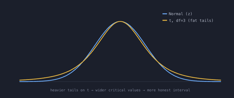
Degrees of freedom and why t becomes z. The t is indexed by df \(= n-1\) (the same \(n{-}1\) from the variance correction).

• Small \(n\): few df, fat tails, t critical values noticeably bigger than z (df=9 gives \(t\approx 2.26\) vs \(z=1.96\)). Wider interval.
• Large \(n\): \(s\) becomes a reliable estimate of \(\sigma\), the extra randomness vanishes, and t converges to the normal. By \(n\approx 30\), t and z are nearly identical.

The honest modern practice: if \(\sigma\) is unknown, always use t. Correct for all \(n\), self-corrects to z for large \(n\).

Situation	Distribution
\(\sigma\) known	z
\(\sigma\) unknown (estimated by \(s\))	t with df \(= n-1\)

What if the data is not normal? Both intervals assumed normal data. What rescues you is, again, the CLT. The machinery needs the sampling distribution of \(\bar x\) to be normal, not the data itself, and the CLT delivers that as \(n\) grows regardless of shape:

• Data normal: z/t intervals exact at any \(n\).
• Non-normal but \(n\) large (at least 30, more if very skewed): CLT kicks in, \(\bar x\) approximately normal, t-interval approximately valid. The everyday situation.
• Non-normal AND \(n\) small: stuck, CLT has not engaged. Options: a transformation (e.g. log), or bootstrapping (resample thousands of times, compute \(\bar x\) each time, read the interval off the empirical distribution, no normality assumption).

CIs for the mean are remarkably robust to non-normality given decent \(n\). They break only when data is both non-normal and small.

Confidence interval for the difference of two means. Often you care about a difference, treatment versus control, A versus B:

\[(\bar x_1-\bar x_2)\;\pm\;t^*\cdot SE_{\text{diff}}, \qquad SE_{\text{diff}}=\sqrt{\frac{s_1^2}{n_1}+\frac{s_2^2}{n_2}}\]

Variances of independent quantities add, hence the square root of summed SEs. Two wrinkles: (1) equal-variance assumption (pooled t) versus not (Welch's t, the safer default, with an approximate df formula); (2) independent samples versus paired (same subjects twice collapses to a one-sample CI on the differences). If the CI for \((\mu_1-\mu_2)\) contains 0, the data is consistent with "no real difference" between the groups. This is the bridge to hypothesis testing.

§8 CIs for Variance & Proportions

Variance, the chi-squared interval. The CI for \(\sigma^2\) breaks the symmetric "plus or minus margin" pattern because the relevant sampling distribution is the chi-squared (\(\chi^2\)), which is skewed, not symmetric. The quantity \((n-1)s^2/\sigma^2\) follows \(\chi^2\) with \(n-1\) df; invert it to bracket \(\sigma^2\):

\[\left(\frac{(n-1)s^2}{\chi^2_{\alpha/2,\,n-1}},\;\; \frac{(n-1)s^2}{\chi^2_{1-\alpha/2,\,n-1}}\right)\]

Two different chi-squared critical values (upper and lower tails) make the interval asymmetric around \(s^2\). Summary: variance goes to chi-squared goes to asymmetric interval, and it strongly assumes normal data (it is not CLT-rescued like the mean).

Proportion, the z interval. For proportion \(p\), the estimate is \(\hat p=\) successes\(/n\), and by the CLT (a proportion is a mean of 0/1 data) it is approximately normal for large \(n\). SE uses \(\hat p\) itself:

\[\hat p \pm z_{\alpha/2}\sqrt{\frac{\hat p(1-\hat p)}{n}}\]

There is no separate \(\sigma\) to estimate, the Bernoulli variance \(p(1-p)\) is fully determined by \(p\), so the t-correction story (extra randomness from estimating \(\sigma\)) does not apply. The catch: the normal approximation needs enough successes and failures, rule of thumb \(n\hat p\ge 10\) and \(n(1-\hat p)\ge 10\); for small samples or extreme \(p\), use Wilson or Clopper-Pearson.

§9 Estimation Reference: The Four Cases

The same ideas organized as a lookup by what you are estimating and the population size.

1, Mean for a large population.

\[\bar x \pm t_{\alpha/2,\,n-1}\cdot\frac{s}{\sqrt n} \qquad (\text{use } z\cdot\sigma/\sqrt n \text{ only if } \sigma \text{ known})\]

\(\text{SE}=s/\sqrt n\). Width shrinks as \(1/\sqrt n\), to halve the margin you need four times the data. Validity rests on normal data or large \(n\) (CLT).

2, Proportion for a large population.

\[\hat p \pm z_{\alpha/2}\sqrt{\frac{\hat p(1-\hat p)}{n}}\]

Uses z. Needs \(n\hat p\ge 10\) and \(n(1-\hat p)\ge 10\). Margin is widest at \(\hat p=0.5\) (maximum uncertainty), why pollsters quote worst-case margins assuming \(p=0.5\).

3, Variance.

\[\left(\frac{(n-1)s^2}{\chi^2_{\alpha/2,\,n-1}},\;\; \frac{(n-1)s^2}{\chi^2_{1-\alpha/2,\,n-1}}\right)\]

Estimator \(s^2=\frac{1}{n-1}\sum(x_i-\bar x)^2\) (the unbiased one). Uses chi-squared with \(n-1\) df, so asymmetric. Strongly assumes normality (not CLT-rescued). For \(\sigma\), take square roots of the endpoints.

4, Proportion for a small, finite population. The case people forget. Standard SE formulas secretly assume an effectively infinite population (sampling with replacement, independent draws). When the population is finite and small and you sample a meaningful fraction without replacement, draws are negatively correlated, each person sampled is one fewer left, which reduces the true uncertainty. You are closer to a census, so you should be more confident. The fix is the Finite Population Correction (FPC):

\[\hat p \pm z_{\alpha/2}\sqrt{\frac{\hat p(1-\hat p)}{n}}\cdot\underbrace{\sqrt{\frac{N-n}{N-1}}}_{\text{FPC}}\]

• \(n\) tiny versus \(N\) (sliver of a huge population): \(N-n\approx N-1\), so FPC \(\approx 1\), no correction, back to the infinite-population formula. Why you ignore FPC for large populations.
• \(n\) approaches \(N\) (sampled nearly everyone): FPC goes to 0, margin of error collapses toward zero, sensible, you have nearly measured the whole population. A census (\(n=N\)) gives FPC = 0: zero sampling error.

Rule of thumb: apply the FPC when the sample is more than about 5% of the population (\(n/N>0.05\)). The same FPC also multiplies the SE for a mean in a small finite population, it is a general standard-error correction, not specific to proportions.

Interview Questions

Q1: When do you use a z interval versus a t interval for a mean, and why? Use a z interval when the population standard deviation \(\sigma\) is known, and a t interval when you estimate it with the sample \(s\). Estimating \(\sigma\) adds a second source of randomness in the denominator, fattening the tails, so the t distribution with \(n-1\) degrees of freedom gives wider, more honest critical values. As \(n\) grows, \(s\) becomes reliable and t converges to z.

Q2: A confidence interval for the difference of two means contains zero. What does that tell you? It tells you the data are consistent with no real difference between the groups, because zero difference is a plausible value within the interval. This is the bridge to hypothesis testing: an interval that excludes zero indicates a detectable difference, while one straddling zero cannot distinguish the groups.

Q3: Why is the confidence interval for a variance asymmetric? Because the relevant sampling distribution, the chi-squared for \((n-1)s^2/\sigma^2\), is skewed rather than symmetric. Inverting it uses two different critical values from the upper and lower tails, which produces an interval that is not symmetric around \(s^2\). It also strongly assumes normal data and is not rescued by the central limit theorem.

Q4: What is the finite population correction and when does it matter? It is the factor \(\sqrt{(N-n)/(N-1)}\) that multiplies the standard error when sampling a meaningful fraction of a small finite population without replacement, since the negatively correlated draws reduce uncertainty. It is near one when the sample is a tiny fraction of the population and goes to zero as the sample approaches a census, and the rule of thumb is to apply it when the sample exceeds about 5% of the population.