Learning Rate Schedules

The learning rate is the single most important hyperparameter. Schedules vary it over training to balance early-stage exploration with late-stage convergence.

Rapid Recall

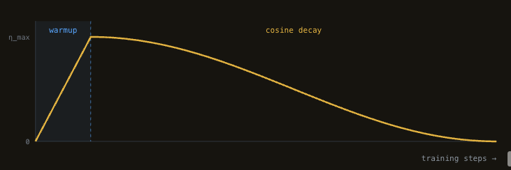
Step decay drops the LR by a factor every \(N\) epochs (classic ResNet, but discontinuous). Cosine annealing decays smoothly from \(\eta_{\max}\) to \(\eta_{\min}\) on a half-cosine and is the CNN-from-scratch default. The transformer standard is warmup + cosine: a linear ramp over the first ~1% of steps, then cosine decay. Warmup exists because gradients are noisy when weights are random, so large early steps push the model into bad regions it cannot escape. ReduceLROnPlateau reacts to a stalled validation loss; one-cycle varies LR up and down. For LLMs, schedule on steps, not epochs.

The transformer-training standard: a short linear warmup ramp up to the peak learning rate, then a smooth cosine decay back toward zero over the rest of training.

§1 Step decay (classical)

Drop the LR by a factor (for example, 10x) every \(N\) epochs.

\[ \eta(\text{epoch}) = \eta_{\text{init}} \cdot \gamma^{\lfloor \text{epoch} / \text{step\_size} \rfloor} \]

Example: lr = 0.1, drop by 10x at epochs 30, 60, 90. Used in original ResNet training. Issue: discontinuous, sudden drops cause loss spikes. Modern schedules avoid this.

§2 Cosine annealing

Smooth decay from \(\eta_{\max}\) to \(\eta_{\min}\) following a half-cosine curve:

\[ \eta(t) = \eta_{\min} + \frac{1}{2}(\eta_{\max} - \eta_{\min})\left(1 + \cos\left(\frac{\pi t}{T}\right)\right) \qquad (t = \text{current step}, \ T = \text{total steps}) \]

Why cosine specifically? Empirical. It tested better than linear decay or exponential decay across many benchmarks. The slow-fast-slow shape (slow at start, fast in the middle, slow at the end) tends to help convergence.

§3 Warmup + cosine (modern LLM standard)

The combination used for transformer training:

\[ \begin{aligned} \textbf{Phase 1 (warmup, first ~1\% of steps):}\quad & \eta \text{ linearly increases from } \approx 0 \text{ to } \eta_{\max} \\ \textbf{Phase 2 (cosine annealing, rest of training):}\quad & \eta \text{ follows the cosine curve from } \eta_{\max} \text{ to } \eta_{\min} \end{aligned} \]

Why warmup?

At step 0, weights are random. Gradient estimates are essentially noise, they don't reliably point toward descent. Large LR updates at this stage push weights into bad regions that are hard to escape. Warmup ramps the LR from near-zero to the target over the first ~1% of steps, letting the model build crude but stable representations before trusting gradients with full-size steps. Once representations are stable, cosine decay smoothly reduces the LR to help the optimizer settle into a sharp minimum. Without warmup, transformers often see loss spikes in the first few hundred steps that the model never recovers from.

Interview-ready warmup answer

"Warmup prevents large initial updates when gradients are noisy and weights have not formed useful representations yet. Once the model has learned something meaningful, the full learning rate is safe to use."

§4 ReduceLROnPlateau (reactive)

Watch validation loss. If it does not improve for patience epochs, multiply the LR by a factor (typically 0.1). Good for unknown problems where you don't know a good schedule a priori. Less common in production where you have already calibrated.

§5 Cyclical / one-cycle (Smith, 2017)

Vary the LR up and down throughout training in cycles. Counterintuitive but works for some tasks. Less common now.

§6 Recommendation matrix

Setting	Schedule
Fine-tuning small model	Constant LR or linear decay
Training CNN from scratch	Cosine annealing
Training transformer / LLM	Warmup + cosine
Unknown problem, want safety	ReduceLROnPlateau
Hyperparameter search	Constant LR (focus on magnitude first)

§7 Implementation (PyTorch)

from torch.optim.lr_scheduler import LinearLR, CosineAnnealingLR, SequentialLR

warmup_steps = 1000
total_steps = 100000

warmup = LinearLR(optimizer, start_factor=0.01, end_factor=1.0, total_iters=warmup_steps)
cosine = CosineAnnealingLR(optimizer, T_max=total_steps - warmup_steps)
scheduler = SequentialLR(optimizer, schedulers=[warmup, cosine], milestones=[warmup_steps])

# In training loop, after optimizer.step():
scheduler.step()

Step-level vs epoch-level: for LLM training, schedule on steps, not epochs (there is often only 1 epoch). For CNN training, epoch-level is fine.

Interview Questions

Q1: Why warmup before cosine decay?

At the start of training, weights are random and haven't formed meaningful representations yet. The gradient estimates are noisy because the model's outputs are near-random. Large learning rate updates at this stage push weights into bad regions that are hard to escape. Warmup ramps the learning rate from near-zero to the target LR over a few thousand steps, letting the model first build crude but stable representations before trusting the gradient direction with large steps. Once training is stable, cosine decay smoothly reduces the LR to help the optimizer settle into a sharp minimum.