Vanishing Gradients

The single equation that explains the problem: the gradient at an early layer is a product of \(L\) per-layer Jacobians. If each factor is consistently below 1, the product collapses exponentially to zero. Early layers stop learning. Everything else in this section is a fix for this.

Rapid Recall

The layer-1 gradient is a chain of \(L\) Jacobians, each roughly \(W_k \cdot \sigma'(z_k)\). With sigmoid, \(\sigma'\) caps at 0.25, so a 10-layer stack shrinks the gradient by at least \(0.25^{10} \approx 10^{-6}\) and early layers stop learning. RNNs are worst hit because the same \(W_h\) is reused at every step, so the product is over time as well as depth. The three fixes are better activations plus initialization (ReLU, He init), the LSTM gradient highway, and residual connections.

§1 The core equation

For an \(L\)-layer network, the gradient at layer 1's weights is a chain of matrix products:

\[ \frac{\partial L}{\partial W_1} = \frac{\partial L}{\partial a_L} \cdot \prod_{k=2}^{L} \frac{\partial a_k}{\partial a_{k-1}} \cdot \frac{\partial a_1}{\partial W_1} \]

Each layer-to-layer Jacobian is approximately:

\[ \frac{\partial a_k}{\partial a_{k-1}} \approx W_k \cdot \sigma'(z_k) \]

The gradient is a chain of \(L\) matrix products. If the magnitude of each factor is consistently less than 1, the product collapses geometrically. If consistently greater than 1, it explodes geometrically. Both are catastrophic.

§2 The sigmoid disaster, numerically

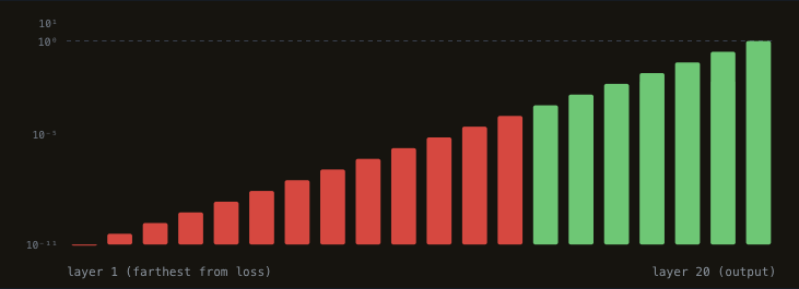
Picture a 20-layer network with sigmoid activations. Max \(\sigma'(z) = 0.25\). Assume weights have spectral norm \(\approx 1\) (generous). Each layer's Jacobian magnitude \(\le 0.25\).

\[ \begin{aligned} \text{Layer 20:}\quad & 0.25^{1} = 2.5 \times 10^{-1} \\ \text{Layer 15:}\quad & 0.25^{6} = 2.4 \times 10^{-4} \\ \text{Layer 10:}\quad & 0.25^{11} = 2.4 \times 10^{-7} \\ \text{Layer 5:}\quad & 0.25^{16} = 2.3 \times 10^{-10} \\ \text{Layer 1:}\quad & 0.25^{20} = 9.1 \times 10^{-13} \end{aligned} \]

By layer 5, the gradient is \(10^{-10}\). Layer 1 receives \(10^{-13}\). Training halts. Early layers cannot learn meaningful features.

Gradient magnitude propagating from the output layer (right) back toward layer 1 (left) on a log scale. With a per-layer factor below 1 (sigmoid ≈ 0.25), the gradient decays geometrically: red bars are the starved early layers, green bars the healthy later ones. A factor of 1.0 (ReLU, stable) keeps the bars level; a factor above 1 makes them explode.

§3 Why this is especially bad in RNNs

An RNN uses the same weight matrix at every time step. The backprop-through-time gradient looks like:

\[ \frac{\partial L}{\partial W} \propto \prod_{t=1}^{T} W_h^{\top} \cdot \mathrm{diag}\big(\sigma'(h_t)\big) \]

If the largest singular value of \(W_h\) is below 1, gradients vanish exponentially over time. Above 1, they explode. Either way you cannot capture long-range dependencies because the gradient connecting time step 100 to time step 1 has either evaporated or blown up. The LSTM gradient highway is the fix.

§4 The three fixes (overview)

Each gets its own treatment elsewhere in this section.

• Better activations + initialization. ReLU (derivative 1 in the active region) avoids the 0.25 cap. He initialization keeps activation variance stable across layers.
• LSTM gradient highway (for RNNs). The cell-state update creates a path through time where gradients flow unattenuated. See gradient highways.
• Residual connections (for deep feedforward / CNN / transformers). Identity-plus-residual creates a gradient bypass. See gradient highways.

Interview Questions

Q1: Why does sigmoid cause vanishing gradients, and how do you fix it?

Sigmoid's derivative is \(\sigma(z)(1-\sigma(z))\), which maxes out at 0.25. In a network with \(L\) layers, the gradient at layer 1 is approximately the product of \(L\) such derivatives. For 10 layers, that's at most \(0.25^{10} \approx 10^{-6}\). Early layers receive essentially zero gradient and stop learning. The fix is ReLU: its derivative is exactly 1 in the active region, so gradients don't shrink as they pass through. For transformers, GELU is preferred because it's smooth and doesn't hard-gate at 0. Residual connections (skip connections) are another key fix, they provide a gradient highway that bypasses the activation functions entirely. He initialization keeps activation variance stable across layers.